Interactive Hover for Big Data#
Interactive Hover for Big Data#
When visualizing large datasets with Datashader, you can easily identify macro level patterns. However, the aggregation process that converts the data into an image can make it difficult to examine individual data points, especially if they occupy the same pixel. This sets up a challenge: how do you explore individual data points without sacrificing the benefits of aggregation?
To solve this problem, HoloViews offers the selector keyword, which makes it possible for the hover tooltip to include information about the underlying data points when using a Datashader operation (rasterize or datashade).
The selector mechanism performantly retrieves the specific details on the server side without having to search through the entire dataset or having to send all the data to the browser. This allows users working with large datasets to detect big picture patterns while also accessing information about individual points.
This notebook demonstrates how to use selector, which creates a dynamic hover tool that keeps the interactive experience fast and smooth with very large datasets and makes it easier to explore and understand complex visualizations.
Note
This notebook uses dynamic updates, which require running a live Jupyter or Bokeh server. When viewed statically, the plots will not update, you can zoom and pan, and hover information will not be available.
Note
This functionality requires Bokeh version 3.7 or greater.
Let’s start by creating a Points element with a DataFrame consisting of five datasets combined. Each of the datasets has a random x, y-coordinate based on a normal distribution centered at a specific (x, y) location, with varying standard deviations. The datasets—labeled d1 through d5—represent different clusters:
d1is tightly clustered around (2, 2) with a small spread of 0.03,d2is around (2, -2) with a wider spread of 0.10,d3is around (-2, -2) with even more dispersion at 0.50,d4is broadly spread around (-2, 2) with a standard deviation of 1.00,and
d5has the widest spread of 3.00 centered at the origin (0, 0).
Each point also carries a val and cat column to identify its dataset and category. The total dataset contains 50,000 points, evenly split across the five distributions.
import datashader as ds
import numpy as np
import pandas as pd

import holoviews as hv
from holoviews.operation.datashader import datashade, dynspread, rasterize

hv.extension("bokeh")

# Set default hover tools on various plot types
hv.opts.defaults(hv.opts.RGB(tools=["hover"]), hv.opts.Image(tools=["hover"]))


def create_synthetic_dataset(x, y, s, val, cat):
    seed = np.random.default_rng(1)
    num = 10_000
    return pd.DataFrame(
        {"x": seed.normal(x, s, num), "y": seed.normal(y, s, num), "s": s, "val": val, "cat": cat}
    )


df = pd.concat(
    {
        cat: create_synthetic_dataset(x, y, s, val, cat)
        for x, y, s, val, cat in [
            (2, 2, 0.03, 0, "d1"),
            (2, -2, 0.10, 1, "d2"),
            (-2, -2, 0.50, 2, "d3"),
            (-2, 2, 1.00, 3, "d4"),
            (0, 0, 3.00, 4, "d5"),
        ]
    },
    ignore_index=True,
)


points = hv.Points(df)

# Show a sample from each dataset
df.iloc[[0, 10_000, 20_000, 30_000, 40_000]]


| x | y | s | val | cat | |
|---|---|---|---|---|---|
| 0 | 2.010368 | 1.982550 | 0.03 | 0 | d1 |
| 10000 | 2.034558 | -2.058168 | 0.10 | 1 | d2 |
| 20000 | -1.827208 | -2.290838 | 0.50 | 2 | d3 |
| 30000 | -1.654416 | 1.418324 | 1.00 | 3 | d4 |
| 40000 | 1.036753 | -1.745027 | 3.00 | 4 | d5 |
Datashader Operations#
Datashader is used to convert the points into a rasterized image. Two common operations are:
rasterize: Converts points into an image grid where each pixel aggregates data. The default is to count the number of points per pixel.datashade: Applies a color map to the rasterized data, outputting RGBA values
The default aggregator counts the points per pixel, but you can specify a different aggregator, for example, ds.mean("s") to calculate the mean of the s column. For more information, see the Large Data user guide.
rasterized = rasterize(points)
shaded = datashade(points)
rasterized + shaded
Selectors are a subtype of Aggregators#
Both aggregator and selector relate to performing an operation on data points in a pixel, but it’s important to understand the difference.
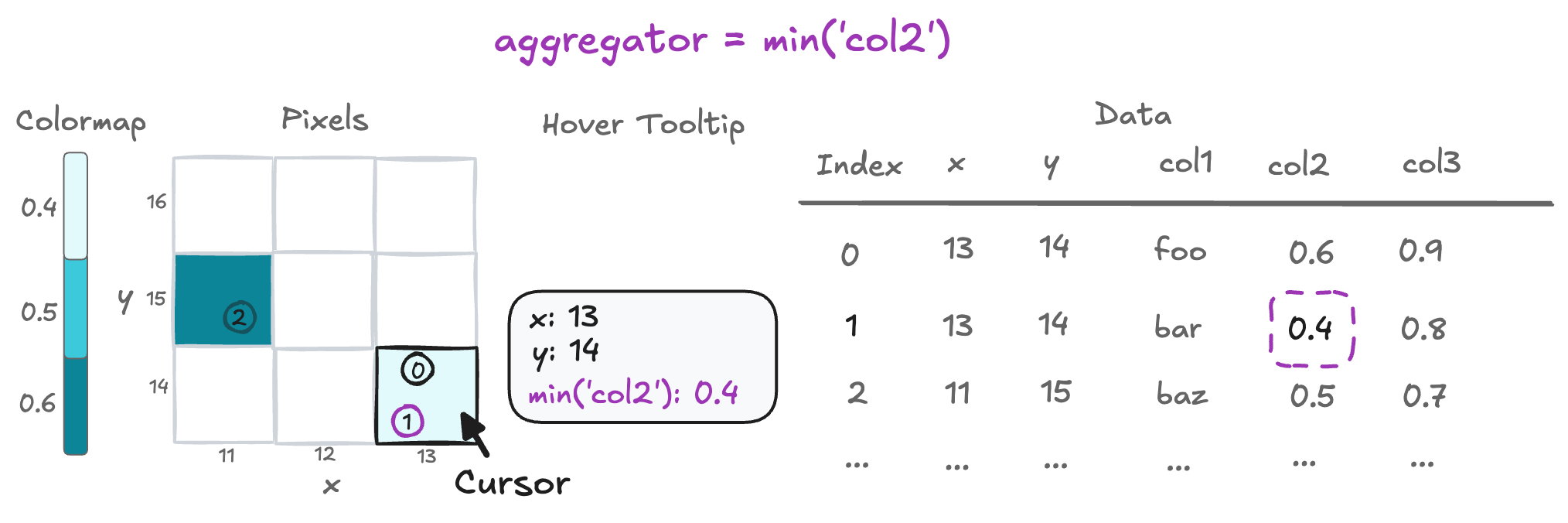
When multiple data points fall into the same pixel, Datashader needs to get a single value from this collection to form an image. This is done with an aggregator that can specify if the points should be combined (such as the mean of a column) or that a single value should just be selected (such as the min of a column).
Let’s see a couple of different aggregators in action:
# Combine data points for the aggregation:
rasterized_mean = rasterize(points, aggregator=ds.mean("s")).opts(title="Aggregate is Mean of s col")

# Select a data point for the aggregation:
rasterized_max = rasterize(points, aggregator=ds.max("s")).opts(title="Aggregate is Max of s column")

rasterized_mean + rasterized_max
Selectors#
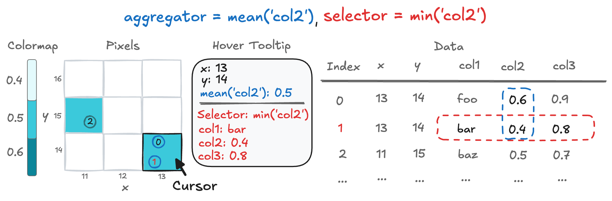
Since a selector is a subtype of aggregator, then why do we need a separate selector keyword? The answer is that very often, users will want to retain hover tooltip information about the particular data point within each pixel (e.g., with min or max) while aggregating the data to form an image using an approach that combines the overlapping data points (e.g., with count or mean). The following are valid selector operations that expose information for the server-side hover tool to collect about one of the underlying data points in a pixel:
ds.min(<column>): Select the row with the minimum value for the columnds.max(<column>): Select the row with the maximum value for the columnds.first(<column>): Select the first value in the columnds.last(<column>): Select the last value in the column
Under the hood, the selected value has a corresponding row-index, which allows the collection and presentation of the entire row in the hover tooltip. If no column is set, the selector will use the index to determine the sample.
Server-side HoverTool#
The key idea behind the server-side HoverTool is:
Hover event: When a user hovers over a plot, the pixel coordinates are sent to the server.
Data lookup: The server uses these coordinates to look up the corresponding aggregated data from the pre-computed dataset.
Update display: The hover information is updated and sent back to the front end to display detailed data.
This design avoids sending all the raw data to the client and only transmits the necessary information on-demand. You can enable this by adding a selector to a rasterize or datashade operation.
By adding an selector we now get the information of all the dimensions in the DataFrame along with the original Hover Information, for this example the new information is s, val, and cat. The new information is split with a horizontal rule.
rasterized_with_selector = rasterize(points, aggregator=ds.mean("s"), selector=ds.min("s"))
rasterized_with_selector
You can specify which columns to show in the HoverTool with hover_tooltips. You can also rename the label by passing in a tuple with (label, column). The information about the selector itself can be disabled by setting selector_in_hovertool=False.
hover_tooltips=["x", "y", ("s [mean(s)]", "x_y s"), ("s [min(s)]", "s"), ("cat [min(s)]", "cat")]
rasterized_with_selector.opts(hover_tooltips=hover_tooltips, selector_in_hovertool=False)
Note
When selector is enabled, hover tooltips use a predefined grid layout with fixed styling, limiting the customization options that would otherwise be available through hover_tooltips in standard plots that don’t utilize selector.
Some useful functions are spread and dynspread, which enhance the visual output by increasing the spread of pixels. This helps make points easier to hover over when zooming in on individual points.
dynspreaded = dynspread(rasterized_with_selector)
rasterized_with_selector + dynspreaded
See also
Large Data: An introduction to Datashader and HoloViews