Gridded Datasets#

import xarray as xr
import numpy as np
import holoviews as hv
from holoviews import opts
hv.extension('matplotlib')

opts.defaults(opts.Scatter3D(color='Value', cmap='fire', edgecolor='black', s=50))

In the Tabular Data guide we covered how to work with columnar data in HoloViews. Apart from tabular or column based data there is another data format that is particularly common in the science and engineering contexts, namely multi-dimensional arrays. The gridded data interfaces allow working with grid-based datasets directly.

Grid-based datasets have two types of dimensions:

they have coordinate or key dimensions, which describe the sampling of each dimension in the value arrays
they have value dimensions which describe the quantity of the multi-dimensional value arrays

There are many different types of gridded datasets, which each approximate or measure a surface or space at discretely specified coordinates. In HoloViews, gridded datasets are typically one of three possible types: Regular rectilinear grids, irregular rectilinear grids, and curvilinear grids. Regular rectilinear grids can be defined by 1D coordinate arrays specifying the spacing along each dimension, while the other types require grid coordinates with the same dimensionality as the underlying value arrays, specifying the full n-dimensional coordinates of the corresponding array value. HoloViews provides many different elements supporting regularly spaced rectilinear grids, but currently only QuadMesh supports irregularly spaced rectilinear and curvilinear grids.

The difference between uniform, rectilinear and curvilinear grids is best illustrated by the figure below:

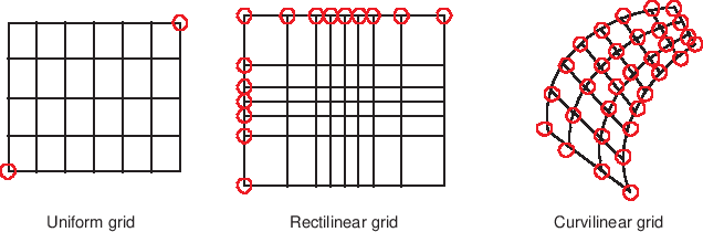
grid-types — Types of logically rectangular grid tiles. Red circles show the values needed to specify grid coordinates for each type. Reproduced from ESMF documentation

In this section we will first discuss how to work with the simpler rectilinear grids and then describe how to define a curvilinear grid with 2D coordinate arrays.

Declaring gridded data#

All Elements that support a ColumnInterface also support the GridInterface. The simplest example of a multi-dimensional (or more precisely 2D) gridded dataset is an image, which has implicit or explicit x-coordinates, y-coordinates and an array representing the values for each combination of these coordinates. Let us start by declaring an Image with explicit x- and y-coordinates:

img = hv.Image((range(10), range(5), np.random.rand(5, 10)), datatype=['grid'])
img

In the above example we defined that there would be 10 samples along the x-axis, 5 samples along the y-axis and then defined a random 5x10 array, matching those dimensions. This follows the NumPy (row, column) indexing convention. When passing a tuple HoloViews will use the first gridded data interface, which stores the coordinates and value arrays as a dictionary mapping the dimension name to a NumPy array representing the data:

img.data

{'x': array([0, 1, 2, 3, 4, 5, 6, 7, 8, 9]),
 'y': array([0, 1, 2, 3, 4]),
 'z': array([[0.47763978, 0.69007192, 0.42700334, 0.50576975, 0.50664489,
         0.14818596, 0.02146588, 0.49242966, 0.14133532, 0.25974912],
        [0.08804022, 0.73240172, 0.94465703, 0.36386923, 0.84061396,
         0.34624043, 0.6642148 , 0.86736984, 0.46485729, 0.41803341],
        [0.53924104, 0.03778663, 0.11950471, 0.56068355, 0.2218625 ,
         0.90082448, 0.16648371, 0.99835878, 0.0114279 , 0.27772819],
        [0.15704396, 0.8846674 , 0.99561018, 0.55110769, 0.02489588,
         0.60650059, 0.05294865, 0.53925873, 0.95024972, 0.24494105],
        [0.69687301, 0.08824034, 0.98070757, 0.64194234, 0.33625406,
         0.05871452, 0.91344753, 0.1579743 , 0.07041152, 0.96407568]])}

However HoloViews also ships with an interface for xarray and the GeoViews library ships with an interface for iris objects, which are two common libraries for working with multi-dimensional datasets:

arr_img = img.clone(datatype=['image'])
print(type(arr_img.data))

try: 
    xr_img = img.clone(datatype=['xarray'])

    print(type(xr_img.data))    
except:
    print('xarray interface could not be imported.')

<class 'numpy.ndarray'>
<class 'xarray.core.dataset.Dataset'>

In the case of an Image HoloViews also has a simple image representation which stores the data as a single array and converts the x- and y-coordinates to a set of bounds:

print("Array type: %s with bounds %s" % (type(arr_img.data), arr_img.bounds))

Array type: <class 'numpy.ndarray'> with bounds BoundingBox(points=((-0.5,-0.5),(9.5,4.5)))

To summarize the constructor accepts a number of formats where the value arrays should always match the shape of the coordinate arrays:

A simple np.ndarray along with (l, b, r, t) bounds
A tuple of the coordinate and value arrays
A dictionary of the coordinate and value arrays indexed by their dimension names
XArray DataArray or XArray Dataset
An Iris cube

Working with a multi-dimensional dataset#

A gridded Dataset may have as many dimensions as desired, however individual Element types only support data of a certain dimensionality. Therefore we usually declare a Dataset to hold our multi-dimensional data and take it from there.

dataset3d = hv.Dataset((range(3), range(5), range(7), np.random.randn(7, 5, 3)),
                       ['x', 'y', 'z'], 'Value')
dataset3d

:Dataset   [x,y,z]   (Value)

This is because even a 3D multi-dimensional array represents volumetric data which we can display easily only if it contains few samples. In this simple case we can get an overview of what this data looks like by casting it to a Scatter3D Element (which will help us visualize the operations we are applying to the data:

hv.Scatter3D(dataset3d)

Indexing#

In order to explore the dataset we therefore often want to define a lower dimensional slice into the array and then convert the dataset:

dataset3d.select(x=1).to(hv.Image, ['y', 'z']) + hv.Scatter3D(dataset3d.select(x=1))

Groupby#

Another common method to apply to our data is to facet or animate the data using groupby operations. HoloViews provides a convenient interface to apply groupby operations and select which dimensions to visualize.

(dataset3d.to(hv.Image, ['y', 'z'], 'Value', ['x']) +
hv.HoloMap({x: hv.Scatter3D(dataset3d.select(x=x)) for x in range(3)}, kdims='x'))

Aggregating#

Another common operation is to aggregate the data with a function thereby reducing a dimension. You can either aggregate the data by passing the dimensions to aggregate or reduce a specific dimension. Both have the same function:

hv.Image(dataset3d.aggregate(['x', 'y'], np.mean)) + hv.Image(dataset3d.reduce(z=np.mean))

By aggregating the data we can reduce it to any number of dimensions we want. We can for example compute the spread of values for each z-coordinate and plot it using a Spread and Curve Element. We simply aggregate by that dimension and pass the aggregation functions we want to apply:

hv.Spread(dataset3d.aggregate('z', np.mean, np.std)) * hv.Curve(dataset3d.aggregate('z', np.mean))

It is also possible to generate lower-dimensional views into the dataset which can be useful to summarize the statistics of the data along a particular dimension. A simple example is a box-whisker of the Value for each x-coordinate. Using the .to conversion interface we declare that we want a BoxWhisker Element indexed by the x dimension showing the Value dimension. Additionally we have to ensure to set groupby to an empty list because by default the interface will group over any remaining dimension.

dataset3d.to(hv.BoxWhisker, 'x', 'Value', groupby=[])

Similarly we can generate a Distribution Element showing the Value dimension, group by the ‘x’ dimension and then overlay the distributions, giving us another statistical summary of the data:

dataset3d.to(hv.Distribution, 'Value', [], groupby='x').overlay()

Categorical dimensions#

The key dimensions of the multi-dimensional arrays do not have to represent continuous values, we can display datasets with categorical variables as a HeatMap Element:

heatmap = hv.HeatMap((['A', 'B', 'C'], ['a', 'b', 'c', 'd', 'e'], np.random.rand(5, 3)))
heatmap + hv.Table(heatmap)

Non-uniform rectilinear grids#

As discussed above, there are two main types of grids handled by HoloViews. So far, we have mainly dealt with uniform, rectilinear grids, but we can use the QuadMesh element to work with non-uniform rectilinear grids and curvilinear grids.

In order to define a non-uniform, rectilinear grid we can declare explicit irregularly spaced x- and y-coordinates. In the example below we specify the x/y-coordinate bin edges of the grid as arrays of shape M+1 and N+1 and a value array (zs) of shape NxM:

n = 8  # Number of bins in each direction
xs = np.logspace(1, 3, n)
ys = np.linspace(1, 10, n)
zs = np.arange((n-1)**2).reshape(n-1, n-1)
print('Shape of x-coordinates:', xs.shape)
print('Shape of y-coordinates:', ys.shape)
print('Shape of value array:', zs.shape)
hv.QuadMesh((xs, ys, zs))

Shape of x-coordinates: (8,)
Shape of y-coordinates: (8,)
Shape of value array: (7, 7)

Curvilinear grids#

To define a curvilinear grid the x/y-coordinates of the grid should be defined as 2D arrays of shape NxM or N+1xM+1, i.e. either as the bin centers or the bin edges of each 2D bin.

n=20
coords = np.linspace(-1.5,1.5,n)
X,Y = np.meshgrid(coords, coords);
Qx = np.cos(Y) - np.cos(X)
Qy = np.sin(Y) + np.sin(X)
Z = np.sqrt(X**2 + Y**2)

print('Shape of x-coordinates:', Qx.shape)
print('Shape of y-coordinates:', Qy.shape)
print('Shape of value array:', Z.shape)

qmesh = hv.QuadMesh((Qx, Qy, Z))
qmesh

Shape of x-coordinates: (20, 20)
Shape of y-coordinates: (20, 20)
Shape of value array: (20, 20)

API#

Accessing the data#

In order to be able to work with data in different formats Holoviews defines a general interface to access the data. The dimension_values method allows returning underlying arrays.

Key dimensions (coordinates)#

By default dimension_values will return the expanded columnar format of the data:

heatmap.dimension_values('x')

array(['A', 'A', 'A', 'A', 'A', 'B', 'B', 'B', 'B', 'B', 'C', 'C', 'C',
       'C', 'C'], dtype='<U1')

To access just the unique coordinates along a dimension simply supply the expanded=False keyword:

heatmap.dimension_values('x', expanded=False)

array(['A', 'B', 'C'], dtype='<U1')

Finally we can also get a non-flattened, expanded coordinate array returning a coordinate array of the same shape as the value arrays

heatmap.dimension_values('x', flat=False)

array([['A', 'B', 'C'],
       ['A', 'B', 'C'],
       ['A', 'B', 'C'],
       ['A', 'B', 'C'],
       ['A', 'B', 'C']], dtype='<U1')

Value dimensions#

When accessing a value dimension the method will similarly return a flat view of the data:

heatmap.dimension_values('z')

array([0.20401146, 0.74194112, 0.47378148, 0.19197437, 0.20709886,
       0.55806993, 0.71113221, 0.04770358, 0.26015043, 0.14215156,
       0.7702703 , 0.42459429, 0.77482621, 0.15832747, 0.56909708])

We can pass the flat=False argument to access the multi-dimensional array:

heatmap.dimension_values('z', flat=False)

array([[0.20401146, 0.55806993, 0.7702703 ],
       [0.74194112, 0.71113221, 0.42459429],
       [0.47378148, 0.04770358, 0.77482621],
       [0.19197437, 0.26015043, 0.15832747],
       [0.20709886, 0.14215156, 0.56909708]])

This web page was generated from a Jupyter notebook and not all interactivity will work on this website. Right click to download and run locally for full Python-backed interactivity.