Deploying Bokeh Apps#
import numpy as np
import holoviews as hv
hv.extension('bokeh')
Purpose#
HoloViews is an incredibly convenient way of working interactively and exploratively within a notebook or commandline context. However, once you have implemented a polished interactive dashboard or some other complex interactive visualization, you will often want to deploy it outside the notebook to share with others who may not be comfortable with the notebook interface.
In the simplest case, to visualize some HoloViews container or element obj, you can export it to a standalone HTML file for sharing using the save function of the Bokeh renderer:
hv.save(obj, 'out.html')
This command will generate a file out.html that you can put on any web server, email directly to colleagues, etc.; it is fully self-contained and does not require any Python server to be installed or running.
Unfortunately, a static approach like this cannot support any HoloViews object that uses DynamicMap (either directly or via operations that return DynamicMaps like decimate, datashade, and rasterize). Anything with DynamicMap requires a live, running Python server to dynamically select and provide the data for the various parameters that can be selected by the user. Luckily, when you need a live Python process during the visualization, the Bokeh server provides a very convenient way of deploying HoloViews plots and interactive dashboards in a scalable and flexible manner. The Bokeh server allows all the usual interactions that HoloViews lets you define and more including:
responding to plot events and tool interactions via Linked Streams
generating and interacting with plots via the usual widgets that HoloViews supports for HoloMap and DynamicMap objects.
using periodic and timeout events to drive plot updates
combining HoloViews plots with custom Bokeh plots to quickly write highly customized apps.
Overview#
In this guide we will cover how we can deploy a Bokeh app from a HoloViews plot in a number of different ways:
Inline from within the Jupyter notebook
Starting a server interactively and open it in a new browser window.
From a standalone script file
Combining HoloViews and Bokeh models to create a more customized app
If you have read a bit about HoloViews you will know that HoloViews objects are not themselves plots, instead they contain sufficient data and metadata allowing them to be rendered automatically in a notebook context. In other words, when a HoloViews object is evaluated a backend specific Renderer converts the HoloViews object into Bokeh models, a Matplotlib figure or a Plotly graph. This intermediate representation is then rendered as an image or as HTML with associated Javascript, which is what ends up being displayed.
The workflow#
The most convenient way to work with HoloViews is to iteratively improve a visualization in the notebook. Once you have developed a visualization or dashboard that you would like to deploy you can use the BokehRenderer to export the visualization as illustrated above, or you can deploy it as a Bokeh server app.
Here we will create a small interactive plot, using Linked Streams, which mirrors the points selected using box- and lasso-select tools in a second plot and computes some statistics:
# Declare some points
points = hv.Points(np.random.randn(1000,2 ))

# Declare points as source of selection stream
selection = hv.streams.Selection1D(source=points)

# Write function that uses the selection indices to slice points and compute stats
def selected_info(index):
    arr = points.array()[index]
    if index:
        label = 'Mean x, y: %.3f, %.3f' % tuple(arr.mean(axis=0))
    else:
        label = 'No selection'
    return points.clone(arr, label=label).opts(color='red')

# Combine points and DynamicMap
selected_points = hv.DynamicMap(selected_info, streams=[selection])
layout = points.opts(tools=['box_select', 'lasso_select']) + selected_points

layout
Working with the BokehRenderer#
When working with Bokeh server or wanting to manipulate a backend specific plot object you will have to use a HoloViews Renderer directly to convert the HoloViews object into the backend specific representation. Therefore we will start by getting a hold of a BokehRenderer:
renderer = hv.renderer('bokeh')
print(renderer)
BokehRenderer()
All Renderer classes in HoloViews are so called ParameterizedFunctions; they provide both classmethods and instance methods to render an object. You can easily create a new Renderer instance using the .instance method:
renderer = renderer.instance(mode='server')
Renderers can also have different modes. In this case we will instantiate the renderer in 'server' mode, which tells the Renderer to render the HoloViews object to a format that can easily be deployed as a server app. Before going into more detail about deploying server apps we will quickly remind ourselves how the renderer turns HoloViews objects into Bokeh models.
Figures#
The BokehRenderer converts the HoloViews object to a HoloViews Plot, which holds the Bokeh models that will be rendered to screen. As a very simple example we can convert a HoloViews Image to a HoloViews plot:
plot = renderer.get_plot(layout)
print(plot)
<LayoutPlot LayoutPlot01811>
Using the state attribute on the HoloViews plot we can access the Bokeh Column model, which we can then work with directly.
plot.state
Column(id=’1570’, …)
In the background this is how HoloViews converts any HoloViews object into Bokeh models, which can then be converted to embeddable or standalone HTML and be rendered in the browser. This conversion is usually done in the background using the figure_data method:
html = renderer._figure_data(plot, 'html')
Bokeh Documents#
In Bokeh the Document is the basic unit at which Bokeh models (such as plots, layouts and widgets) are held and serialized. The serialized JSON representation is then sent to BokehJS on the client-side browser. When in 'server' mode the BokehRenderer will automatically return a server Document:
renderer(layout)
(<bokeh.document.Document at 0x11afc7590>,
 {'file-ext': 'html', 'mime_type': u'text/html'})
We can also easily use the server_doc method to get a Bokeh Document, which does not require you to make an instance in ‘server’ mode.
doc = renderer.server_doc(layout)
doc.title = 'HoloViews App'
In the background however, HoloViews uses the Panel library to render components to a Bokeh model which can be rendered in the notebook, to a file or on a server:
import panel as pn

model = pn.panel(layout).get_root()
model
For more information on the interaction between Panel and HoloViews see the the Panel documentation.
Deploying with panel serve#
Deployment from a script with panel serve is one of the most common ways to deploy a Bokeh app. Any .py or .ipynb file that attaches a plot to Bokeh’s curdoc can be deployed using panel serve. The easiest way to do this is using wrapping the HoloViews component in Panel using pn.panel(hvobj) and then calling the panel_obj.servable() method, which accepts any HoloViews object ensures that the plot is discoverable by Panel and the underlying Bokeh server. See below to see a full standalone script:
import numpy as np
import panel as pn
import holoviews as hv
import holoviews.plotting.bokeh

points = hv.Points(np.random.randn(1000,2 )).opts(tools=['box_select', 'lasso_select'])
selection = hv.streams.Selection1D(source=points)

def selected_info(index):
    arr = points.array()[index]
    if index:
        label = 'Mean x, y: %.3f, %.3f' % tuple(arr.mean(axis=0))
    else:
        label = 'No selection'
    return points.clone(arr, label=label).opts(color='red')

layout = points + hv.DynamicMap(selected_info, streams=[selection])

pn.panel(layout).servable(title='HoloViews App')
In just a few steps we can iteratively refine in the notebook to a deployable Panel app. Note also that we can also deploy an app directly from a notebook. By using .servable() in a notebook any regular .ipynb file can be made into a valid Panel/Bokeh app, which can be served with panel serve example.ipynb.
It is also possible to create a Bokeh Document more directly working with the underlying Bokeh representation instead. This in itself is sufficient to make the plot servable using bokeh serve:
hv.renderer('bokeh').server_doc(layout)
In addition to starting a server from a script we can also start up a server interactively, so let’s do a quick deep dive into Bokeh Application and Server objects and how we can work with them from within HoloViews.
Bokeh Server#
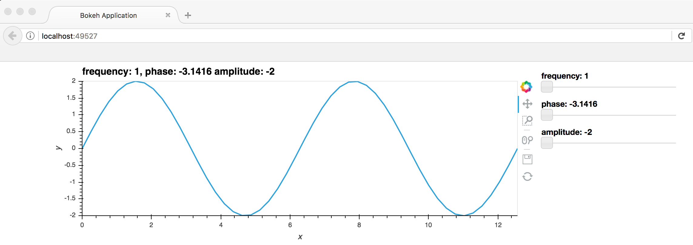
To start a Bokeh server directly from a notebook we can also use Panel, specifically we’ll use the panel.serve function. We’ll define a DynamicMap of a sine Curve varying by frequency, phase and an offset and then create a server instance using Panel:
def sine(frequency, phase, amplitude):
    xs = np.linspace(0, np.pi*4)
    return hv.Curve((xs, np.sin(frequency*xs+phase)*amplitude)).opts(width=800)

ranges = dict(frequency=(1, 5), phase=(-np.pi, np.pi), amplitude=(-2, 2), y=(-2, 2))
dmap = hv.DynamicMap(sine, kdims=['frequency', 'phase', 'amplitude']).redim.range(**ranges)

server = pn.serve(dmap, start=False, show=False)
<bokeh.server.server.Server object at 0x10b3a0510>
Next we can define a callback on the IOLoop that will open the server app in a new browser window and actually start the app (and if outside the notebook the IOLoop):
server.start()
server.show('/')

# Outside the notebook ioloop needs to be started
# from tornado.ioloop import IOLoop
# loop = IOLoop.current()
# loop.start()
After running the cell above you should have noticed a new browser window popping up displaying our plot. Once you are done playing with it you can stop it with:
server.stop()
We can achieve the equivalent using the .show method on a Panel object:
server = pn.panel(dmap).show()
We will once again stop this Server before continuing:
server.stop()
Inlining apps in the notebook#
Instead of displaying our app in a new browser window we can also display an app inline in the notebook simply by using the .app method on Panel object. The server app will be killed whenever you rerun or delete the cell that contains the output. Additionally, if your Jupyter Notebook server is not running on the default address or port (localhost:8888) supply the websocket origin, which should match the first part of the URL of your notebook:
dmap
Periodic callbacks#
One of the most important features of deploying apps is the ability to attach asynchronous, periodic callbacks, which update the plot. The simplest way of achieving this is to attach a Counter stream on the plot which is incremented on each callback. As a simple demo we’ll simply compute a phase offset from the counter value, animating the sine wave:
def sine(counter):
    phase = counter*0.1%np.pi*2
    xs = np.linspace(0, np.pi*4)
    return hv.Curve((xs, np.sin(xs+phase))).opts(width=800)

counter = hv.streams.Counter()
hv.DynamicMap(sine, streams=[counter])

dmap
Once we have created a Panel object we can call the add_periodic_callback method to set up a periodic callback. The first argument to the method is the callback and the second argument period specified in milliseconds. As soon as we start this callback you should see the Curve above become animated.
def update():
    counter.event(counter=counter.counter+1)

cb = pn.state.add_periodic_callback(update, period=200)
Once started we can stop and start it at will using the .stop and .start methods:
cb.stop()
Combining Bokeh Application and Flask Application#
While Panel and Bokeh are great ways to create an application often we want to leverage the simplicity of a Flask server. With Flask we can easily embed a HoloViews, Bokeh and Panel application in a regular website. The main idea for getting Bokeh and Flask to work together is to run both apps on ports and then use Flask to pull the Bokeh Serve session with pull_session from bokeh.client.session.
def sine(frequency, phase, amplitude):
    xs = np.linspace(0, np.pi*4)
    return hv.Curve((xs, np.sin(frequency*xs+phase)*amplitude)).options(width=800)

ranges = dict(frequency=(1, 5), phase=(-np.pi, np.pi), amplitude=(-2, 2), y=(-2, 2))
dmap = hv.DynamicMap(sine, kdims=['frequency', 'phase', 'amplitude']).redim.range(**ranges)

pn.serve(dmap, websocket_origin='localhost:5000', port=5006, show=False)
We run load up our dynamic map into a Bokeh Application with the parameter allow_websocket_origin=["localhost:5000"]
from bokeh.client import pull_session
from bokeh.embed import server_session
from flask import Flask, render_template
from flask import send_from_directory

app = Flask(__name__)


# locally creates a page
@app.route('/')
def index():
    with pull_session(url="http://localhost:5006/") as session:
        # generate a script to load the customized session
        script = server_session(session_id=session.id, url='http://localhost:5006')
        # use the script in the rendered page
    return render_template("embed.html", script=script, template="Flask")

if __name__ == '__main__':
    # runs app in debug mode
    app.run(port=5000, debug=True)
Note that in a notebook context we cannot use pull_session but this example demonstrates how we can embed the Bokeh server inside a simple flask app.
This is an example of a basic flask app. To find out more about Flask a tutorial can be found on the Flask Quickstart Guide.
Below is an example of a basic Flask App that pulls from the Bokeh Application. The Bokeh Application is using Server from Bokeh and IOLoop from tornado to run the app.
# holoviews.py

import holoviews as hv
import panel as pn
import numpy as np

hv.extension('bokeh')

def sine(frequency, phase, amplitude):
    xs = np.linspace(0, np.pi*4)
    return hv.Curve((xs, np.sin(frequency*xs+phase)*amplitude)).options(width=800)

if __name__ == '__main__':
    ranges = dict(frequency=(1, 5), phase=(-np.pi, np.pi), amplitude=(-2, 2), y=(-2, 2))
    dmap = hv.DynamicMap(sine, kdims=['frequency', 'phase', 'amplitude']).redim.range(**ranges)
    pn.serve(dmap, port=5006, allow_websocket_origin=["localhost:5000"], show=False)
#flaskApp.py

from bokeh.client import pull_session
from bokeh.embed import server_session
from flask import Flask, render_template
from flask import send_from_directory

app = Flask(__name__)

# locally creates a page
@app.route('/')
def index():
    with pull_session(url="http://localhost:5006/") as session:
            # generate a script to load the customized session
            script = server_session(session_id=session.id, url='http://localhost:5006')
            # use the script in the rendered page
    return render_template("embed.html", script=script, template="Flask")


if __name__ == '__main__':
    # runs app in debug mode
    app.run(port=5000, debug=True)
<!-- embed.html -->

<!doctype html>

<html lang="en">
<head>
  <meta charset="utf-8">
  <title>Embedding a Bokeh Server With Flask</title>
</head>

<body>
  <div>
    This Bokeh app below served by a Bokeh server that has been embedded
    in another web app framework. For more information see the section
    <a  target="_blank" href="https://bokeh.pydata.org/en/latest/docs/user_guide/server.html#embedding-bokeh-server-as-a-library">Embedding Bokeh Server as a Library</a>
    in the User's Guide.
  </div>
  {{ script|safe }}
</body>
</html>
If you wish to replicate navigate to the examples/gallery/apps/flask directory and follow the these steps:
Step One: call
python holoviews_app.pyin the terminal (this will start the Panel/Bokeh server)Step Two: open a new terminal and call
python flask_app.py(this will start the Flask application)Step Three: go to web browser and type
localhost:5000and the app will appear
Combining HoloViews and Panel or Bokeh Plots/Widgets#
While HoloViews provides very convenient ways of creating an app it is not as fully featured as Bokeh itself is. Therefore we often want to extend a HoloViews based app with Panel or Bokeh plots and widgets. Here we will discover to achieve this with both Panel and then the equivalent using pure Bokeh.
import holoviews as hv
import numpy as np
import panel as pn

# Create the holoviews app again
def sine(phase):
    xs = np.linspace(0, np.pi*4)
    return hv.Curve((xs, np.sin(xs+phase))).opts(width=800)

stream = hv.streams.Stream.define('Phase', phase=0.)()
dmap = hv.DynamicMap(sine, streams=[stream])

start, end = 0, np.pi*2
slider = pn.widgets.FloatSlider(start=start, end=end, value=start, step=0.2, name="Phase")

# Create a slider and play buttons
def animate_update():
    year = slider.value + 0.2
    if year > end:
        year = start
    slider.value = year

def slider_update(event):
    # Notify the HoloViews stream of the slider update
    stream.event(phase=event.new)

slider.param.watch(slider_update, 'value')

def animate(event):
    if button.name == '► Play':
        button.name = '❚❚ Pause'
        callback.start()
    else:
        button.name = '► Play'
        callback.stop()

button = pn.widgets.Button(name='► Play', width=60, align='end')
button.on_click(animate)
callback = pn.state.add_periodic_callback(animate_update, 50, start=False)

app = pn.Column(
    dmap,
    pn.Row(slider, button)
)

app
If instead we want to deploy this we could add .servable as discussed before or use pn.serve. Note however that when using pn.serve all sessions will share the same state therefore it is best to
wrap the creation of the app in a function which we can then provide to pn.serve. For more detail on deploying Panel applications also see the Panel server deployment guide.
Now we can reimplement the same example using Bokeh allowing us to compare and contrast the approaches:
import numpy as np
import holoviews as hv

from bokeh.io import show, curdoc
from bokeh.layouts import layout
from bokeh.models import Slider, Button

renderer = hv.renderer('bokeh').instance(mode='server')

# Create the holoviews app again
def sine(phase):
    xs = np.linspace(0, np.pi*4)
    return hv.Curve((xs, np.sin(xs+phase))).opts(width=800)

stream = hv.streams.Stream.define('Phase', phase=0.)()
dmap = hv.DynamicMap(sine, streams=[stream])

# Define valid function for FunctionHandler
# when deploying as script, simply attach to curdoc
def modify_doc(doc):
    # Create HoloViews plot and attach the document
    hvplot = renderer.get_plot(dmap, doc)

    # Create a slider and play buttons
    def animate_update():
        year = slider.value + 0.2
        if year > end:
            year = start
        slider.value = year

    def slider_update(attrname, old, new):
        # Notify the HoloViews stream of the slider update
        stream.event(phase=new)

    start, end = 0, np.pi*2
    slider = Slider(start=start, end=end, value=start, step=0.2, title="Phase")
    slider.on_change('value', slider_update)

    callback_id = None

    def animate():
        global callback_id
        if button.label == '► Play':
            button.label = '❚❚ Pause'
            callback_id = doc.add_periodic_callback(animate_update, 50)
        else:
            button.label = '► Play'
            doc.remove_periodic_callback(callback_id)
    button = Button(label='► Play', width=60)
    button.on_click(animate)

    # Combine the holoviews plot and widgets in a layout
    plot = layout([
    [hvplot.state],
    [slider, button]], sizing_mode='fixed')

    doc.add_root(plot)
    return doc

# To display in the notebook
show(modify_doc, notebook_url='localhost:8888')

# To display in a script
#    doc = modify_doc(curdoc())
As you can see depending on your needs you have complete freedom whether to use just HoloViews and deploy your application, combine it Panel or even with pure Bokeh.